Loss Function
Loss(Cost) Function
개요
FYR:
- Loss Funcition
- Classification Loss Funcition
- Regression Loss Funcition
- Sequence Loss Funcition
- Generative Loss Funcition
- Weight Regularization
- Learning Rate
- Learning Rate Scheduler
- Cost Funcition
Loss(Cost) function 이란, 기계학습과 딥러닝에서 모델이 예측한 출력값과 실제 정답 값 사이의 차이를 측정하는 함수이다.
Loss function 은 모델의 예측 성능을 수치적으로 표현하며, 모델이 학습하는 동안 이를 최소화하는 방향으로 매개변수(weight, bias)를 조정한다.
Loss Fn. 의 역할
모델의 성능 평가
- 손실 함수의 주요 역할은 모델의 예측 오류를 수치(수량)화 하는 것.
- 이를 통해 모델은 예측 값과 실제 값 사이의 차이를 바탕으로 얼마나 잘못 예측되었는 지 평가할 수 있다.
- I.e., 모델의 성능이 좋은지 또는, 나쁜지에 대한 정량적 평가 기준 요소가 된다.
최적화된 목표 설정
- 모델의 학습 주요 목표는 Loss value 를 최소화 하는 것이다.
- 손실 함수는 모델이 예측하는 값과, 실제 값 간의 차이를 수치적으로 계산해 주기 때문에
- 최적화 알고리즘(E.g., gradient descent) 는 이 값을 최소화 하는 방향으로 bias 와 weight 를 업데이트한다.
- I.e., Loss function 은 모델이 어떤 방향으로 학습해야하는 지 지시하는 역할을 수행한다.
Loss Fn. 의 중요성
학습 방향 설정
- Loss function 은 모델의 학습 방향을 결정한다.
- Gradient descent 와 같은 최적화 알고리즘이 손실 함수의 값을 줄이는 방향으로 모델을 업데이트 하기 때문에
- 잘 정의된 loss function 은 모델이 효과적으로 학습할 수 있도록 유도한다.
성능 개선을 위한 가이드
- Loss function 은 모델의 성능을 개선하는 데 핵심적인 가이드 역할을 수행한다.
- 손실 값이 클수록 모델의 예측 실제 값과 더 멀리 떨어져있음을 의미하기 때문에,
- 이를 최소화 하는 것이 모델의 성능을 개선하는 데 중요한 목표가 된다.
문제 유형에 따른 맞춤 설계
- Loss function 은 문제의 유형에 따라 적절하게 선택되고 설계되어야 한다.
- Regression 모델에서는 MSE(Mean Squared Error), Classification 모델에서는 Cross-Entropy 와 같은 손실 함수가 적합하다.
- 적절한 loss function 을 선택하지 않으면, 모델이 문제를 효과적으로 해결하지 못하거나 학습이 제대로 이루어지지 않을 수 있다.
Over-Fitting 방지
- 잘 설계된 loss function 은 모델이 훈련 데이터에 over-fitting(과적합) 되지 않도록 유도한다.
- E.g., L2, L1 normalization 과 같은 추가적인 항을 loss function 에 포함시켜, 모델이 지나치게 복잡해 지지 않도록 제어할 수 있다.
다양한 문제에 적용, 해결 가능
- 데이터 분포, 이상치 존재 여부, 클래스 불균형 등 데이터 특성에 따라 적절한 loss function 사용 가능
- E.g., regression 또는 classification 모델에서는 각기 다른 loss function 을 사용하는 것이 좋고,
- 이상치에 강건한 Huber loss, 클래스 불 균형을 다루기 위한 Focal loss 와 같이 다양한 함수는 문제에 따라 더 효과적인 성능을 발휘하도록 유도할 수 있다.
Fundamental Concept
Visualization
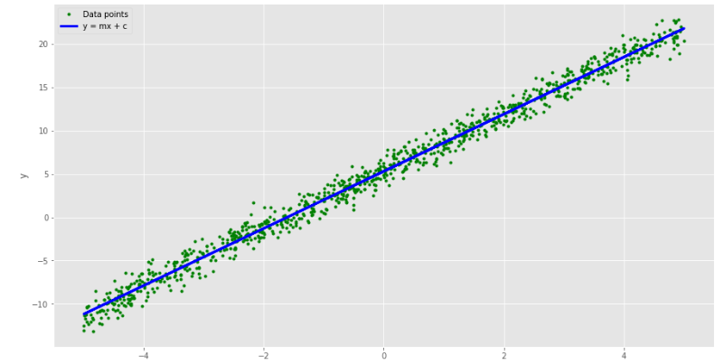
import torch
import matplotlib.pyplot as plt
%matplotlib inline

plt.style.use('ggplot')

plt.rcParams["figure.figsize"] = (15, 8)

# Generating y = mx + c + random noise
num_data = 1000

# True values of m and c
m_line = 3.3
c_line = 5.3

# input (Generate random data between [-5,5])
x = 10 * torch.rand(num_data) - 5

# Output (Generate data assuming y = mx + c + noise)
y_label = m_line * x + c_line + torch.randn_like(x)
y = m_line * x + c_line

# Plot the generated data points
plt.plot(x, y_label, '.', color='g', label="Data points")
plt.plot(x, y, color='b', label='y = mx + c', linewidth=3)
plt.ylabel('y')
plt.xlabel('x')
plt.legend()
plt.show()
Result
Key-Point
The gole is to predict some value of $x$,
To do this we will fit a line that goes through the data points $(x_i,y_i)$.
The equation for such a line is
$y=mx+c$
We have a ser of data points $(x_i,y_i)$, and they should all satisfy the equation above.
I.e.,
$y_i=mx_i+c$
Unless we have perfact data with no noise,
even the best $m$ and $c$ we can fin will not perfectly fit the data.
So, we will have an error or residual given by
$e_i= (y_i - m x_i - c)$
We want to find a value of $m$ and $c$ that minimizes the error above.
Positive or negative values of error are equally bad for us.
So, we are interested in minimizing the square of the error above.
In addition, we want to minimize the squared error over all the data points.
In other words, we want to minimize a function of the residual that tkaes the following form
$l_{sse}=\sum^{N}_{i=1}(y_i-mx_i-c)^2$
This function is called the Loss Function.
The sum of squared errors is just one type of loss function.
Another extenstion of this can be the mean squared error function
which is given by
$l_{mse}=\frac{1}{N}\sum^{N}_{i=1}(y_i-mx_i-c)^2$
- Referenced with OpenCV

Leave a comment